이진화

출처 : http://docs.opencv.org/trunk/d7/d4d/tutorial_py_thresholding.html#gsc.tab=0

 

Adaptive Thresholding

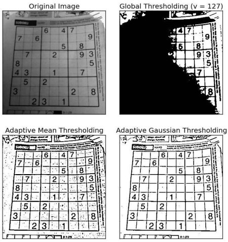
In the previous section, we used a global value as threshold value. But it may not be good in all the conditions where image has different lighting conditions in different areas. In that case, we go for adaptive thresholding. In this, the algorithm calculate the threshold for a small regions of the image. So we get different thresholds for different regions of the same image and it gives us better results for images with varying illumination.

It has three ‘special’ input params and only one output argument.

Adaptive Method - It decides how thresholding value is calculated.

• cv2.ADAPTIVE_THRESH_MEAN_C : threshold value is the mean of neighbourhood area.
• cv2.ADAPTIVE_THRESH_GAUSSIAN_C : threshold value is the weighted sum of neighbourhood values where weights are a gaussian window.

Block Size - It decides the size of neighbourhood area.

C - It is just a constant which is subtracted from the mean or weighted mean calculated.

Below piece of code compares global thresholding and adaptive thresholding for an image with varying illumination:

1 import cv2

2 import numpy as np

3 from matplotlib import pyplot as plt

4 

5 img = cv2.imread('dave.jpg',0)

6 img = cv2.medianBlur(img,5)

7 

8 ret,th1 = cv2.threshold(img,127,255,cv2.THRESH_BINARY)

9 th2 = cv2.adaptiveThreshold(img,255,cv2.ADAPTIVE_THRESH_MEAN_C,\

10  cv2.THRESH_BINARY,11,2)

11 th3 = cv2.adaptiveThreshold(img,255,cv2.ADAPTIVE_THRESH_GAUSSIAN_C,\

12  cv2.THRESH_BINARY,11,2)

13 

14 titles = ['Original Image', 'Global Thresholding (v = 127)',

15  'Adaptive Mean Thresholding', 'Adaptive Gaussian Thresholding']

16 images = [img, th1, th2, th3]

17 

18 for i in xrange(4):

19  plt.subplot(2,2,i+1),plt.imshow(images[i],'gray')

20  plt.title(titles[i])

21  plt.xticks([]),plt.yticks([])

22 plt.show()

Result :

image

Otsu’s Binarization

In the first section, I told you there is a second parameter retVal. Its use comes when we go for Otsu’s Binarization. So what is it?

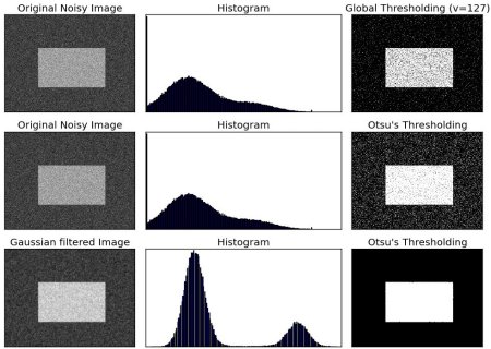
In global thresholding, we used an arbitrary value for threshold value, right? So, how can we know a value we selected is good or not? Answer is, trial and error method. But consider a bimodal image (In simple words, bimodal image is an image whose histogram has two peaks). For that image, we can approximately take a value in the middle of those peaks as threshold value, right ? That is what Otsu binarization does. So in simple words, it automatically calculates a threshold value from image histogram for a bimodal image. (For images which are not bimodal, binarization won’t be accurate.)

For this, our cv2.threshold() function is used, but pass an extra flag, cv2.THRESH_OTSU. For threshold value, simply pass zero. Then the algorithm finds the optimal threshold value and returns you as the second output, retVal. If Otsu thresholding is not used, retVal is same as the threshold value you used.

Check out below example. Input image is a noisy image. In first case, I applied global thresholding for a value of 127. In second case, I applied Otsu’s thresholding directly. In third case, I filtered image with a 5x5 gaussian kernel to remove the noise, then applied Otsu thresholding. See how noise filtering improves the result.

1 import cv2

2 import numpy as np

3 from matplotlib import pyplot as plt

4 

5 img = cv2.imread('noisy2.png',0)

6 

7 # global thresholding

8 ret1,th1 = cv2.threshold(img,127,255,cv2.THRESH_BINARY)

9 

10 # Otsu's thresholding

11 ret2,th2 = cv2.threshold(img,0,255,cv2.THRESH_BINARY+cv2.THRESH_OTSU)

12 

13 # Otsu's thresholding after Gaussian filtering

14 blur = cv2.GaussianBlur(img,(5,5),0)

15 ret3,th3 = cv2.threshold(blur,0,255,cv2.THRESH_BINARY+cv2.THRESH_OTSU)

16 

17 # plot all the images and their histograms

18 images = [img, 0, th1,

19  img, 0, th2,

20  blur, 0, th3]

21 titles = ['Original Noisy Image','Histogram','Global Thresholding (v=127)',

22  'Original Noisy Image','Histogram',"Otsu's Thresholding",

23  'Gaussian filtered Image','Histogram',"Otsu's Thresholding"]

24 

25 for i in xrange(3):

26  plt.subplot(3,3,i*3+1),plt.imshow(images[i*3],'gray')

27  plt.title(titles[i*3]), plt.xticks([]), plt.yticks([])

28  plt.subplot(3,3,i*3+2),plt.hist(images[i*3].ravel(),256)

29  plt.title(titles[i*3+1]), plt.xticks([]), plt.yticks([])

30  plt.subplot(3,3,i*3+3),plt.imshow(images[i*3+2],'gray')

31  plt.title(titles[i*3+2]), plt.xticks([]), plt.yticks([])

32 plt.show()

Result :

image

How Otsu's Binarization Works?

This section demonstrates a Python implementation of Otsu's binarization to show how it works actually. If you are not interested, you can skip this.

Since we are working with bimodal images, Otsu's algorithm tries to find a threshold value (t) which minimizes the weighted within-class variance given by the relation :

σ 2 w (t)=q 1 (t)σ 2 1 (t)+q 2 (t)σ 2 2 (t) 

 

where

q 1 (t)=∑ i=1 t P(i)&q 1 (t)=∑ i=t+1 I P(i) 

 

μ 1 (t)=∑ i=1 t iP(i)q 1 (t) &μ 2 (t)=∑ i=t+1 I iP(i)q 2 (t)  

 

σ 2 1 (t)=∑ i=1 t [i−μ 1 (t)] 2 P(i)q 1 (t) &σ 2 2 (t)=∑ i=t+1 I [i−μ 1 (t)] 2 P(i)q 2 (t)